Introduction

At the time of writing, it is about thirty years since Altman and Bland (1983, 1986) proposed their method to compare two methods of measurement. The development and popularity of this method have been entertainingly described by Bland and Altman (2012). In this article, among other things, they write "It is a great pity that limits of agreement are often stated without their confidence intervals". This is one of several topics we shall explain in the following material, which is intended to assist those who use our software to analyse their data.

Multiple measurements in an subject

When comparing two methods of measurement, it is usual to take pairs of measurements, one in each pair taken with the two different methods. This is particularly likely if the quantity to be measured is unlikely to have a truly constant value, such as heart rate (in contrast to a quantity such as height (at least in the short term). If several pairs of measurements are taken from each subject, this data structure has to be taken into account during the analysis, by applying the appropriate methods. Otherwise,

1. the variance of the differences is underestimated, which means that
2. the limits of agreement (LoA) will are too narrow; and this means
3. the variance of the bias is seriously underestimated; and also
4. the variance of the limits of agreement is seriously underestimated, so finally
5. the 95% confidence intervals (CI) are too narrow.

How much each of these statistics are underestimated depends on the degree of between-subjects variability. If variation between subjects is ignored (usually an incorrect thing to do), the analysis will have a "pooled data" approach. Unless between-subjects variation is known, then errors that result from the "pooled data" approach cannot be known. Recent articles by Bland and Altman (2007) and Myles (2007) emphasize how between-subjects variation leads to underestimation of the limits of agreement. However this is only one effect of between-subjects variation. In addition to smaller limits of agreement there is also substantial underestimation of the 95% confidence intervals of these limits, as emphasized by Hamilton and Davies (2010).

If we would perform a standard Bland-Altman analysis for the first four subjects of the example data, we would obtain the following graph, where the red lines represent the LoA, and the dark red lines the 95% CI for the LoA (range -2.15 to 2.09):

However, if we take into account that these data are actually ten measurements in each of just four subjects, we would obtain the following graph, where especially the 95% CI are much larger (range -6.68 to 6.63):

This is an extreme case, but it demonstrates that the between-subjects variance cannot be precisely estimated from a small number of subjects. Bland and Altman (2012) state that it is not hard to calculate to the confidence intervals. However these calculations are not trivial, and at present there is no dedicated software, apart from the SAS macro by Zou (2013).

Differences should be independent and normally distributed

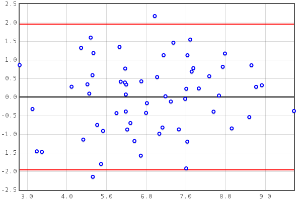
The variance of the differences should not depend on the mean value. this may be visually inspected by observing the (studentized) residuals versus mean plot:

In the above plot, the distribution of the residuals (in the Y direction) does not seem to be dependent on the mean values (X direction). But if heteroscedasticity is visible, a transformation of the data may be used, see Altman and Bland (1983).
Spearman's rank correlation coefficient (ρ, between the ranks of the differences and the means) is given, with its 95% confidence interval. The analysis remains valid if there is an important correlation, but less useful, because the variance of the differences at a specific mean value will be smaller than calculated.

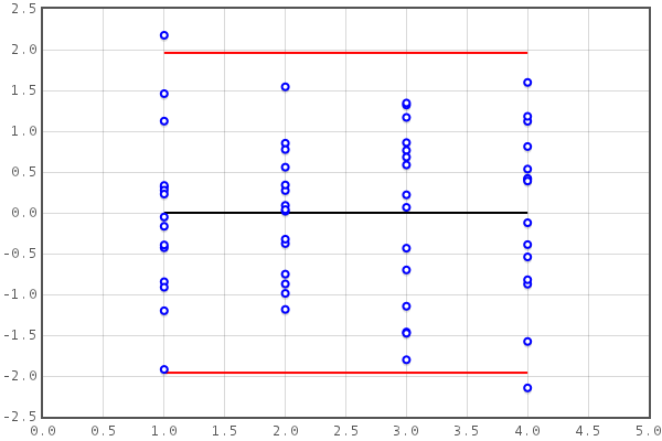
Furthermore, the variance of the differences should not vary between individuals. This may be visually inspected by observing the residuals versus subject ID plot:

In the above plot, the distribution of the residuals does not seem to be dependent on the subject numbers. See Bland and Altman (2007) for further discussion.

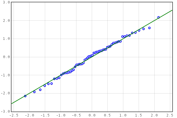
Q-Q plots may be visually inspected to assess the normality of the distributions underlying the differences:

The quantiles of the differences are plotted versus the quantiles of the normal distribution. If these lie close to the line of identity, the distribution of the differences may be approximated by the normal distribution. Outliers may be detected if there are a few points far from the line of identity.

A nonparametric analysis is performed as well. The bias and LoA are then defined as the 50, and 2.5 and 97.5% percentiles, and with a bootstrap procedure their 95% confidence intervals are estimated. Usually, the LoA and especially their CI will not be as accurate as obtained from the parametric analysis. However, discrepancies between the parametric and nonparametric approaches may indicate problems with the data, such as outliers.

Choice of analysis method

The "True value varies" method should always be used (see the manuscript). The "True value constant" method does give some additional information on repeatability (see below). These analyses are automatically carried out and the results are shown below the data form. Analyses performed here can only be used to compare methods, e.g., to demonstrate the differences when the "Pooled data" method is applied.

Results provided on the analysis page

• From the differences of the Y-X data, the bias, or grand mean is calculated. The standard error of the mean (after the +/- sign) is calculated according to the analysis method, and these may therefore differ between methods. With the "Pooled data" method, the standard error is usually underestimated if there is interindividual variability in the bias.
• The SD is the estimated standard deviation of the differences.
• From the mean and 1.96 times the SD, the limits of agreement (LoA) are calculated. For the "Analysis of means" method, these are usually smaller, because they represent the limits of a mean quantity rather than the quantity (difference) itself.
• For the grand mean and the limits of agreement (LoA), 95% confidence intervals are estimated. This is done using approximations, assuming that sums of squares are independent chi-squared variates, using the MOVER, and using the bootstrap (for validation purposes). The MOVER 95% confidence intervals for the LoA are plotted.
• For the "True value varies" and "True value constant" methods, parts of standard ANOVA tables are given. These show the within subject variance (WSV), the between-subjects variance (BSV), and its associated F and P values. If the between-subjects variance of the bias is small, the P value will be high, and results of the different methods similar. The ratio of between-subjects variance and the total variance is given as τ. When τ > 1/3, modifications to the "True value varies" method as described in the paper are applied.
• For the "True value constant" method, the standard deviations of the WSVs, needed to calculate the repeatability coefficients as discussed in Bland and Altman's 1999 paper, are given as SX and SY. Using the MOVER, a 95% CI is calculated for their ratio, which may provide evidence that one measurement device is more precise. The overall means are given as reference values for interpreting the repeatability coefficients.
• Spearman's rank correlation coefficient ρ is given with its 95% CI, based on a bootstrap procedure. This indicates if there is a trend in the bias over the range of values measured.

Results to be reported in a paper

1. The mean of the differences (bias) and the limits of agreement, with their 95% confidence intervals.
2. The standard deviation of the differences with its SE.
3. The within subject variance (WSV) and the between-subjects variance (BSV) or the intraclass correlation τ, with their/its SE, because that indicates that between-subjects variability was estimated.
4. Repeatability coefficients which indicate the precision of the measurement devices.
5. Remarks on visual inspection of the diagnostic plots - these may be shown or reported to be adequate.

Analysis of data containing one measurement per subject

The methods described above estimate both within subject and between-subjects variability, which is not possible when the data contain just one measurement for each subject. Rather than letting the methods fail, this situation is detected and the data are handled accordingly (see Carkeet (2015)).

Literature

DG Altman and JM Bland, Measurement in medicine: the analysis of method comparison studies. The Statistician 1983; 32:307-317.
JM Bland and DG Altman, Statistical methods for assessing agreement between two methods of clinical measurement. Lancet 1986; i:307-310.
JM Bland and DG Altman, Measuring agreement in method comparison studies, Statistical Methods in Medical Research 1999; 8:135-160.
JM Bland and DG Altman, Agreement between methods of measurement with multiple observations per individual, Journal of Biopharmaceutical Statistics 2007; 17:571-582.
JM Bland and DG Altman, Agreed statistics: measurement method comparison, Anesthesiology 2012; 116:182-185.
A Carkeet, Exact Parametric Confidence Intervals for Bland-Altman Limits of Agreement, Optometry and Vision Science 2015.
C Hamilton and S Lewis, The importance of using the correct bounds on the Bland-Altman limits of agreement when multiple measurements are recorded per patient, Journal of Clinical Monitoring and Computing 2010: 24:163-175.
PS Myles, Using the Bland-Altman method to measure agreement with repeated measures (Editorial), British Journal of Anaesthesia 2007; 99:309-311.
GY Zou, Confidence interval estimation for the Bland-Altman limits of agreement with multiple observations per individual, Stat Methods Med Res 2013; 22: 630-642.

Contact

Send comments to Erik Olofsen.